Understanding Language Models 2: Stable Features and Identifiable Causal Structure

A stable feature basis is the prerequisite for interpretable causal structure: first demand run-to-run consistency, then recover temporal and instantaneous relations.

Recap

In the previous post, I argued that mechanistic interpretability (MI) and causal representation learning (CRL) are best viewed as complementary ways of studying the same object: learned computation. MI typically starts from the transformer substrate and searches for circuits; CRL starts from latent variables and asks when their causal structure is identifiable.

That discussion was mostly conceptual. This follow-up is more concrete. I focus on two recent papers that, taken together, suggest a practical ordering for the field. The first argues that SAE-based interpretability should treat feature consistency across training runs as a first-class objective . The second shows how to move beyond isolated features by learning time-delayed and instantaneous causal relations among them, with explicit identifiability guarantees and a scalable implementation for LLM activations .

Read together, the message is simple:

Before we ask for causal structure over features, we should first ask whether the features themselves are stable enough to count as scientific objects.

Why Feature Consistency Comes First

Sparse autoencoders (SAEs) are often used as a candidate coordinate system for language model internals. The hope is that they recover reusable, reasonably monosemantic features that can serve as the basic units of analysis for later work on circuits, steering, or causal interventions.

But there is an obvious concern: if two SAE runs trained on the same activations produce materially different dictionaries, then a feature-level explanation may be little more than an artifact of initialization. In that case, even a compelling-looking circuit story is hard to treat as cumulative knowledge.

Figure 1: Feature consistency is the difference between treating SAE outputs as seed-dependent artifacts and treating them as reusable scientific objects. The desired outcome is alignment across runs up to permutation and scaling, not merely good reconstruction in each run separately.

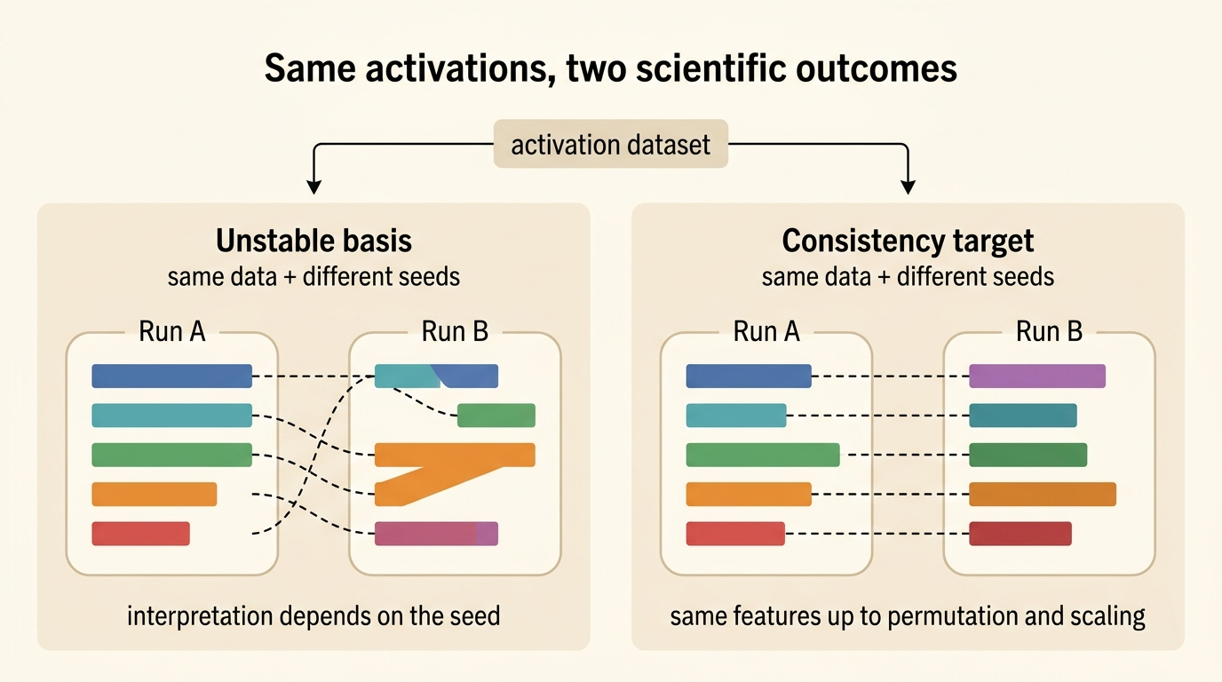
The feature consistency paper sharpens this concern into a methodological claim . Its central proposal is that MI should explicitly measure whether independently trained SAEs converge to the same feature set, up to a permissible equivalence relation. The strongest version considered in the paper is essentially:

\[f_i^{(A)} \approx c_i f_{\pi(i)}^{(B)},\]

meaning that feature dictionaries from two runs should align up to a permutation \(\pi\) and per-feature rescaling coefficients \(c_i\).

To make this operational, the paper advocates Pairwise Dictionary Mean Correlation Coefficient (PW-MCC) as a practical run-to-run consistency metric. This matters for at least three reasons.

1. Reproducibility. If feature dictionaries drift unpredictably across seeds, then discovered features and circuits become difficult to reproduce.
2. Research efficiency. Stable coordinates make it easier to compare methods, reuse annotations, and build on earlier results instead of re-interpreting every run from scratch.
3. Trustworthiness. Consistency is not a full causal guarantee, but it is a necessary condition if we want to treat a recovered feature as more than a convenient visualization.

A compact way to say it: feature consistency is identifiability pressure in practice. If the coordinate system can rotate, split, or absorb arbitrarily from run to run, then feature-level claims are not yet stable scientific claims.

What the Consistency Paper Adds

What I find most useful about the paper is that it does not stop at a vague call for reproducibility. It offers a fairly complete argument across theory, synthetic data, and real LLM activations.

First, it connects SAE consistency to overcomplete sparse dictionary learning. The key theoretical idea is that sparsity can restore uniqueness even when the dictionary is overcomplete. In the paper’s analysis, TopK-style SAEs are especially attractive because exact \(k\)-sparsity and a suitable round-trip property connect naturally to the spark-style conditions that support uniqueness of sparse factorizations. In the ideal matched setting, this yields strong feature consistency up to the familiar permutation-and-scaling ambiguities .

Second, the synthetic experiments show that PW-MCC tracks ground-truth recovery quite well. This is important because on real LLM activations we do not have access to the true latent dictionary. If PW-MCC behaves similarly to the ground-truth MCC in controlled settings, it becomes a useful proxy rather than a purely cosmetic metric.

Third, the real-data experiments show that feature consistency is not merely aspirational. With suitable architectural choices, especially TopK SAEs, high run-to-run consistency appears achievable on actual language model activations. Just as importantly, higher PW-MCC is reported to correlate strongly with the semantic similarity of feature explanations, which suggests that the metric is not detached from what interpretability researchers informally care about.

The broader lesson is not that one metric or one SAE architecture has “solved” the problem. Rather, the field should treat stability of the feature basis as a standard evaluation axis, alongside reconstruction quality, sparsity, and downstream usefulness.

From Isolated Features to Causal Structure

Suppose we grant the first paper its main point. We now have a more stable feature basis. What should we do with it?

Standard SAE workflows mostly answer the question, “Which concepts are present in this activation?” They are much less explicit about relations between concepts. But language is sequential, and many meaningful dependencies are relational rather than unary. A feature may influence another feature in later tokens, and multiple features may constrain one another within the same token.

This is where the second paper enters . It proposes a temporal causal representation model for LLM activations that augments the usual linear-feature view with two distinct kinds of structure:

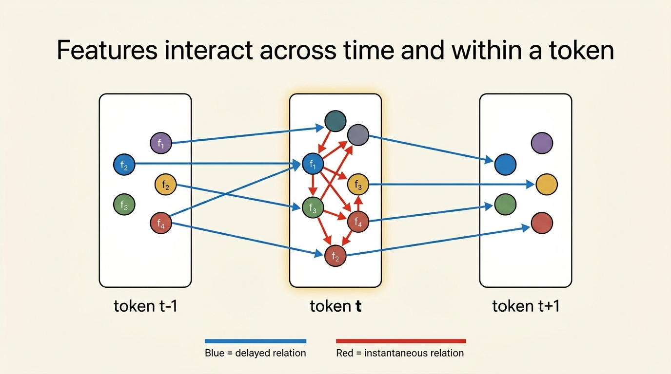
1. Time-delayed relations, which describe how latent concepts at earlier tokens influence concepts at later tokens.
2. Instantaneous relations, which describe same-token dependencies such as co-occurrence, mutual constraint, or local compositional structure.

The conceptual move is straightforward but important. Instead of treating SAE features as independent coordinates, the paper models them as latent variables in a linear temporal structural equation model. Observed activations are still generated from latent concepts through a linear mixing map, but the latent concepts themselves now follow sparse delayed and instantaneous dependencies. In other words, the representation is no longer just a dictionary; it becomes a dynamic causal model.

Figure 2: The temporal-instantaneous view adds structure on top of a feature basis. Blue arrows represent delayed influence across positions, while red arrows represent same-token dependencies such as co-occurrence, exclusion, or local compositional coupling.

The progression is: features give us candidate variables; causal structure tells us how those variables constrain one another across time and within a token.

Why the Temporal-Instantaneous Model Matters

The motivation for this paper is not only expressive power but also identifiability at scale. Existing CRL methods for temporal and instantaneous structure often rely on Jacobian-heavy computations that do not scale well to the thousands of features common in LLM analysis. The paper responds by adopting a linear model and exploiting the autocovariance structure instead.

This choice is restrictive, but it buys something valuable: a theory that is explicit about its assumptions and computationally feasible at the scale of real activations. Under conditions such as temporally white and independent innovations, rank sufficiency, process stability, and non-Gaussianity, the paper characterizes the remaining ambiguities of the recovered model. With additional sparsity and support assumptions, these ambiguities collapse further to familiar component-wise or subspace-level indeterminacies that interpretability researchers know how to reason about .

Operationally, the resulting estimator has three pieces:

1. A linear autoencoding step for reconstructing observations.
2. An independent-noise estimation step for recovering the latent residual structure.
3. Sparse regularization over both delayed and instantaneous adjacency matrices.

This is a nice example of the MI/CRL bridge becoming concrete. The autoencoder part looks familiar from SAE-style representation learning; the independent noise modeling and sparsity-constrained structure recovery come from CRL.

What the Paper Finds on Real Activations

The synthetic and semi-synthetic experiments are important because they show the method can recover the intended latent variables and dependency structure when the data-generating process is known or partially controlled. But for this series, the more interesting part is its analysis of real LLM activations.

On real text, the paper reports that the learned structure uncovers both delayed and same-token relations that are intuitively meaningful. The examples are revealing:

1. Nationality adjectives to the nouns they modify. Features like “Japanese” or “Italians” show delayed relations to noun features that commonly follow them.
2. Formal content to formal style. Features associated with institutional or official language influence later formal verbs and objective adjectives.
3. Structured local dependencies. Same-token relations appear between month-only features and full-date features, between coding-format signals and coding-format content, and between partially overlapping legal citation features.

I would not read these examples as a complete mechanistic explanation of language modeling. But they do show something that standard SAE inventories often miss: the internal concept space is not just a bag of isolated features. It contains structured dependencies that can be modeled, sparsified, and at least partially identified.

Putting the Two Papers Together

The two papers answer different questions, but they fit together almost perfectly.

Figure 3: A practical workflow suggested by the two papers. Representation learning alone is not enough; stable features provide the basis for structure learning, and interventional tests come after both.

Question	Main object	Main risk	Main remedy
Are the recovered features stable across runs?	feature dictionary	run-to-run arbitrariness	explicit consistency metrics and architectures that favor stable sparse factorizations
Are the relations among those features identifiable?	delayed and instantaneous causal structure	correlational stories without structural guarantees	sparse temporal SEMs with identifiable assumptions and scalable estimation

This yields a more operational version of the argument from the first post.

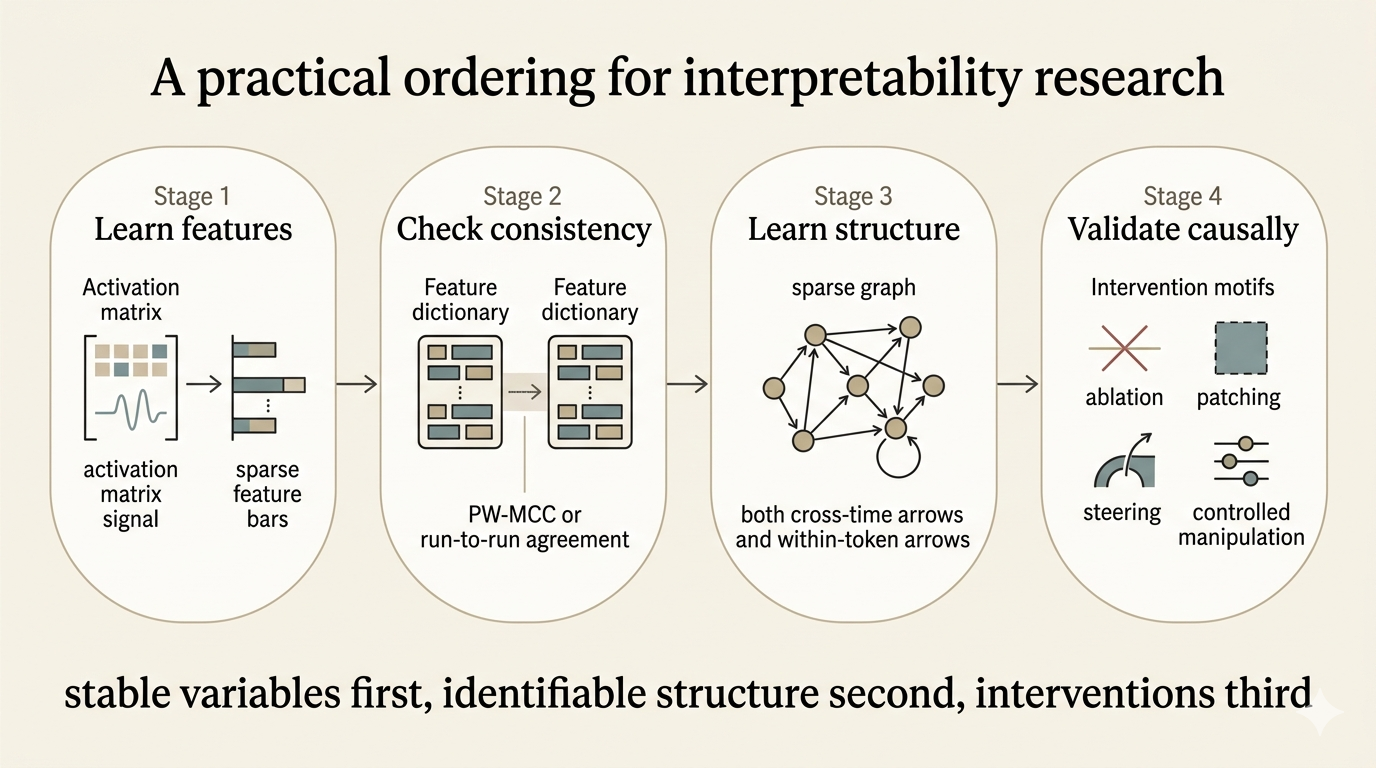
1. Feature extraction: learn a sparse coordinate system for activations.
2. Consistency checking: verify that this coordinate system recurs across runs rather than depending on seed-specific accidents.
3. Structure learning: estimate delayed and instantaneous dependencies among those features under assumptions that make the residual ambiguities explicit.
4. Interventional validation: test whether the discovered variables and edges survive manipulations of the model.

In that sense, the first paper is about the ontology of interpretability: what counts as a stable internal variable? The second is about the causal grammar over that ontology: once variables are stable enough, what relations among them are identifiable?

Summary

If the first post argued that MI and CRL are converging on the same scientific objective, these two papers suggest a concrete research program for that convergence.

First, make the latent feature basis stable enough to trust. Then, on top of that basis, learn causal structure rich enough to describe how concepts interact across time and within tokens. That is a much stronger path than jumping directly from a single SAE run to an ambitious mechanistic story.

My own takeaway is that the field should increasingly think in the following order:

stable variables first, identifiable structure second, interventions third.

That ordering does not solve mechanistic interpretability. But it does make the path forward look more like cumulative science and less like a collection of compelling but fragile anecdotes.

Citation

If you found this post useful, please consider citing it:

@article{song2026understandinglm2,
  title={Understanding Language Models 2: Stable Features and Identifiable Causal Structure},
  author={Song, Xiangchen},
  year={2026},
  month={April},
  url={https://xiangchensong.github.io/blog/2026/understanding-language-models-2/}
}