Understanding Language Models 1: Mechanistic Interpretability Meets Causal Representation Learning

Mechanistic interpretability and causal representation learning study the same object, computation, but from complementary angles: circuits vs variables.

Opening

This is the first post in Understanding Language Models, a short series on opening up the “black box” of LLMs. We do not lack elegant stories about why LLMs behave the way they do; we lack explanations that survive intervention, transfer across contexts, and remain valid out-of-distribution.

The purpose of this post is not to survey mechanistic interpretability (MI) from first principles. Instead, I aim to (i) provide a compact map of contemporary MI practice, and (ii) clarify its conceptual and methodological relationship to causal machine learning—in particular, causal representation learning (CRL). The central claim is that MI and CRL interrogate the same underlying object—learned computation—but they do so at different levels of abstraction: circuits vs variables.

If you have read my earlier CRL posts on sequence models (see #sequence-model), you have seen a recurring theme: learning representations is comparatively easy; identifying the right causal variables is difficult due to identifiability. A closely related issue appears in interpretability: producing a plausible post-hoc “story” is often easy, while obtaining a stable, interventionally valid decomposition is substantially harder.

Motivation: MI and causal machine learning target causal explanations

Figure 1: MI and CRL adopt different abstractions but converge on a shared objective: causal explanations of model behavior. The left branch emphasizes mechanistic circuit discovery in the transformer substrate , while the right branch emphasizes latent-variable DAG structure and identification.

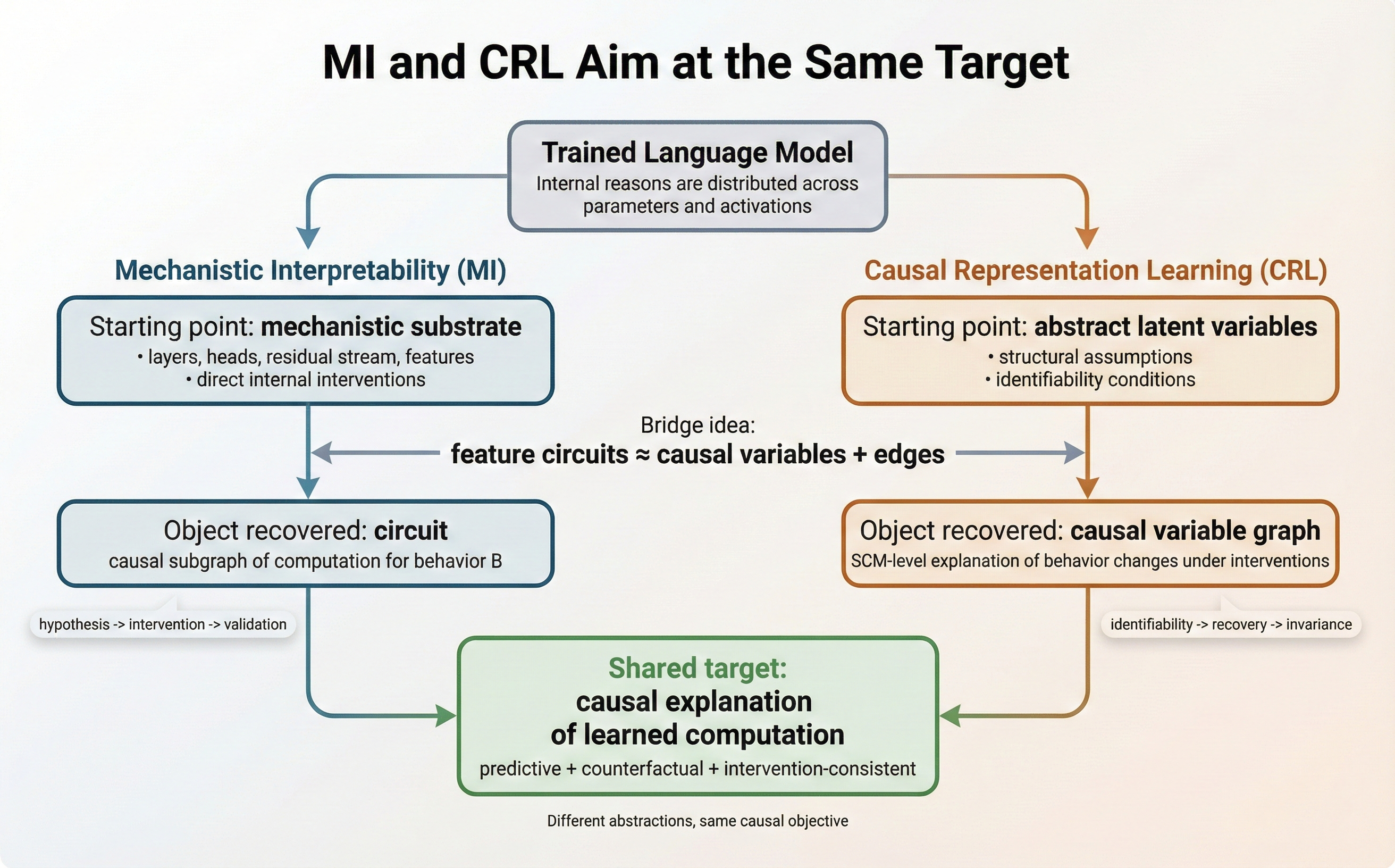
As Figure 1 suggests, MI and causal machine learning can be viewed as two routes to the same endpoint: explanations that are counterfactually meaningful—i.e., they predict how behavior changes under interventions. MI is closer to reverse engineering: start from the transformer substrate and recover sparse functional circuits . Causal machine learning is closer to latent-logic specification: define variables and ask when their causal structure is identifiable. The difference is in the interface, not the intent.

A compact mnemonic: MI starts with the "how" and hunts for the "what"; CRL defines the "what" and checks whether the "how" matches.

Why now: MI has become experimentally tractable

Three developments have pushed mechanistic interpretability (MI) toward a more cumulative, experimentally grounded discipline:

1. Tooling and experimental protocols. It is now standard to cache activations, run patching-style interventions, and instrument models using open tooling (e.g., TransformerLens) . This makes it routine to treat models as systems we can perturb and measure, not just observe.

2. Scaling of causal analyses. The field has moved beyond isolated neuron anecdotes toward feature- and circuit-level explanations with explicit causal tests. Methods such as attribution graphs / circuit tracing aim to scale these analyses to larger models and richer behaviors .

3. A practical basis for scale: SAEs. Sparse autoencoders provide reusable feature coordinates that mitigate the “single-neuron bottleneck” and make circuit discovery more systematic .

Single-neuron bottleneck: neuron-by-neuron interpretation does not scale well and is unstable under superposition. SAEs provide a more reusable feature basis for large-model analysis.

The Linear Representation Hypothesis (as an effective theory)

Most SAE-based workflows assume that residual-stream states are well-approximated by a sparse linear feature basis:

\[x_t^{(\ell)} \approx \sum_{i=1}^m a_{t,i}^{(\ell)} f_i^{(\ell)} .\]

This is consistent with superposition analyses in toy settings and with recent LRH-oriented formulations . But it should be read as a useful modeling assumption, not as proof that the model’s true causal variables are linear. The underlying causal coordinates may live on a nonlinear manifold (e.g., \(z=\phi(x)\) for nonlinear \(\phi\)), in which case linear feature interventions are best understood as an approximation—an effective theory that can still support strong causal tests.

With this framing, many MI projects now follow a recognizable scientific loop:

hypothesis → intervention → behavioral consequence → refinement

This is the logic of causal inference, transposed to instrumented neural networks and increasingly evaluated with explicit counterfactual protocols such as causal scrubbing .

Main idea: “finding the circuit” as a causal explanation of computation

MI is often summarized as “find the circuit.” From a causal machine learning perspective, this slogan can be made precise: a “circuit” is a restricted causal model—a small set of internal variables and mechanisms that are jointly sufficient to explain a target behavior under a specified intervention class.

In contemporary practice, MI typically relies on three coupled abstractions:

1. Units of analysis (features rather than neurons).
   Raw neurons are often polysemantic due to superposition. A growing approach is to use features—directions in activation space extracted via dictionary learning / sparse autoencoders —as more stable and semantically aligned coordinates.

2. Circuits as sparse mechanistic subgraphs.
   A circuit is a small subgraph of transformer computation (heads, MLPs, residual stream components) that is (ideally) both sufficient and close to minimal for the behavior of interest.

3. Causality-first evaluation.
   Explanations are not accepted on correlational evidence alone. They are validated via interventions—ablation, patching, resampling baselines, or steering—designed to isolate necessity/sufficiency relationships.

A useful working hypothesis underlying much of the field is:

Many transformer behaviors are mediated by a relatively small set of reusable mechanisms (“circuits”), which can be recovered by targeted interventions and compactly represented using feature-like units rather than individual neurons.

This claim is empirical rather than theoretical, but it is supported by a growing body of case studies, including induction heads and task-specific circuits such as IOI , among others.

From neurons to features and why causal ML should care

The neuron-level view fails primarily because neurons can participate in multiple unrelated computations (polysemanticity). Feature-based decompositions attempt to provide a coordinate system in which (i) units are more interpretable, and (ii) interventions can be expressed more cleanly (e.g., ablating or steering a feature).

Polysemanticity: one neuron contributes to many concepts. Superposition: many concepts are encoded in overlapping directions, so single-neuron semantics become brittle.

This is precisely the bridge to causal machine learning:

• In causal ML/CRL, we seek latent causal variables that support stable causal generalization.
• In modern MI, extracted features serve as candidate internal variables on which we can intervene.

This motivates a unifying object:

Feature circuits: directed graphs whose nodes are features and whose edges denote causal influence validated by interventions.

The conceptual convergence is that both communities ultimately want variables that are not merely descriptive but interventionally meaningful.

A concrete intuition is the IOI setting: instead of treating an IOI-relevant component as merely a set of active neurons, the CRL view treats it as an operator implementing a causal role (e.g., an S-Inhibition function) within a larger mechanism. This shifts the question from “Which neurons fire?” to “Which causal abstraction is being computed?” .

Circuits vs variables: a translation between MI and causal ML

The following correspondence is often the most useful translation layer:

MI object	Causal ML translation	Practical reading
Feature (SAE direction / residual-stream direction)	Causal variable	features are the alphabet of the causal language
Circuit (sparse mechanistic subgraph)	Causal graph among behavior-relevant variables/mechanisms	MI emphasizes discovery of mechanism
Activation patching / ablation / steering	Interventions (do-operations) on internal variables/mechanisms	shared experimental testbed
“This circuit explains behavior $B$”	Counterfactual claim about behavior under manipulation of $Z$	explanation requires interventional validity

In short: MI emphasizes discovery of internal mechanisms; CRL emphasizes identifiability of variables and edges under assumptions.

This makes the complementarity sharper:

Mechanistic interpretability resembles causal discovery with a known mechanism class (the transformer graph is given),
whereas causal representation learning resembles mechanism discovery with an unknown variable class (the latent variables must be identified).

MI gains leverage from direct surgical access to the computation graph. In CRL, identifiability ensures that discovered variables are not merely one of many fit-the-data explanations, but the unique underlying drivers that persist across distributions. The hard part is Rotational Invariance in residual representations: if \(x=WA\), then for any invertible rotation \(R\) we also have \(x=(WR)(R^{-1}A)\), yielding alternative but behaviorally equivalent coordinates. This helps explain why identifiability is often the hardest problem in LLM internals. Accordingly, sparsity in SAEs is not just a technical convenience; it is the Identifiability Constraint that lets us prefer one coordinate system over an infinite family of rotated alternatives.

Citation

If you found this post useful, please consider citing it:

@article{song2026understandinglm1,
  title={Understanding Language Models 1: Mechanistic Interpretability Meets Causal Representation Learning},
  author={Song, Xiangchen},
  year={2026},
  month={February},
  url={https://xiangchensong.github.io/blog/2026/understanding-language-models-1/}
}