Sequence Model 4: Nonstationary Dynamics

Extending identifiability for sequence models to nonstationary dynamics.

Recap and Motivation

In this series, we study identifiability of sequence models — the question of whether we can provably recover the true latent variables that generated the observed data, rather than learning an arbitrary representation that merely reconstructs observations well. In Sequence Model 1, we formalized this problem. In Sequence Model 2, we introduced sufficient variability, a condition on how much the latent distributions must change across contexts to enable recovery. In Sequence Model 3, we showed that using the history as the context variable, a sequence model can be identifiable.

In all previous posts, the latent causal dynamics \(\mathbf{z}_t = f(\mathbf{z}_{t-1})\) were always assumed to follow a fixed transition function \(f\). In other words, the rules that determine how latent states evolve do not change over time.

In practice, real-world sequences are rarely stationary. A robot’s dynamics change as its joints wear out, economic relationships shift across policy regimes, and a patient’s physiological responses vary as a disease progresses. If the transition function itself changes over time, our previous identifiability results no longer directly apply.

Figure 1: Stationary vs. nonstationary dynamics in a sequence model.

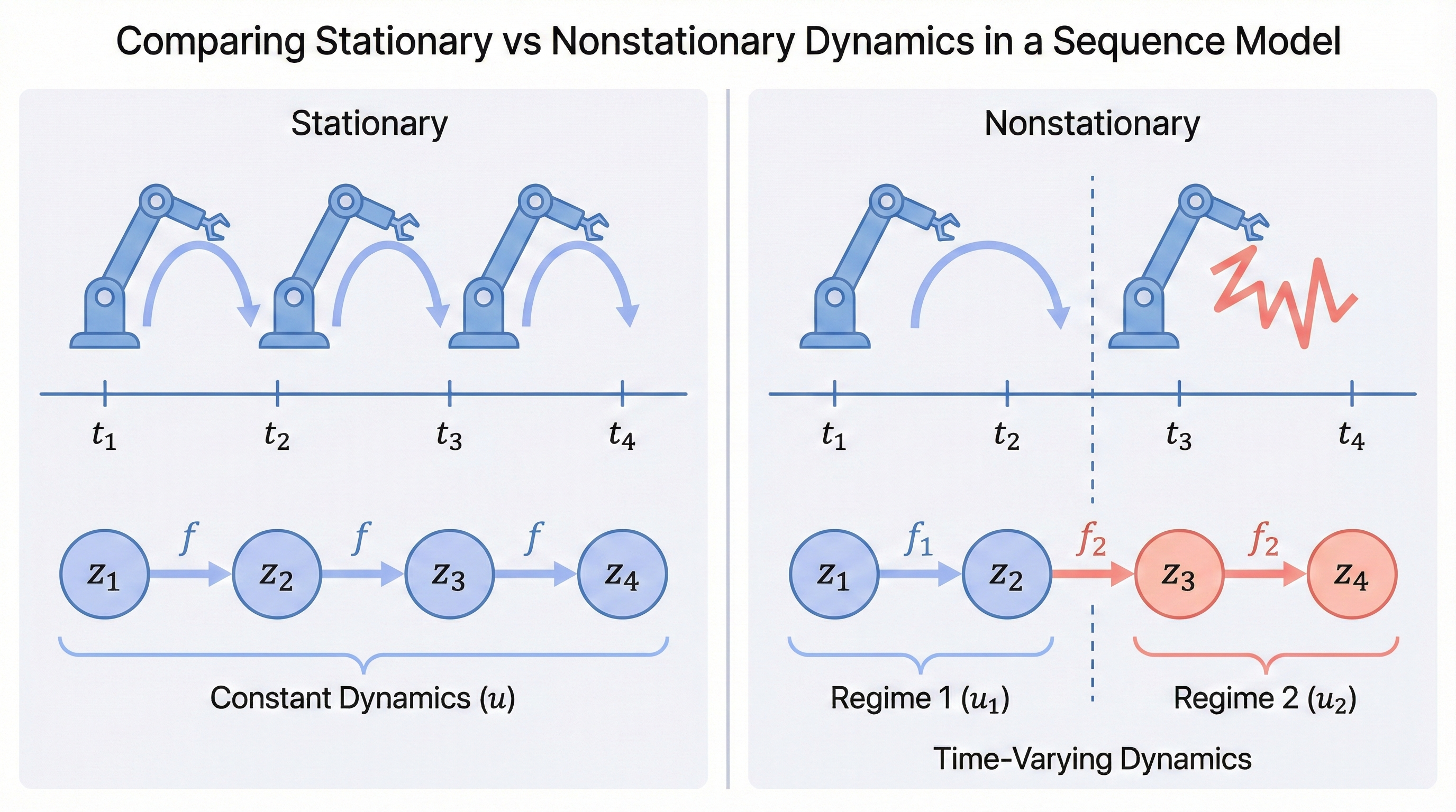
When the transition function is nonstationary, an intuitive approach is: if we can recover the regime variable \(u_t\) — a discrete label indicating which dynamical rule is active at time \(t\) — then we can apply our previous identifiability results within each regime separately.

Markov-Switching Models: A First Attempt

The first approach is fairly straightforward. In sequence modeling, we have a well-established framework for handling hidden changing regimes: the Hidden Markov Model (HMM), where a discrete latent state evolves via a Markov chain and each state emits an observation. If we further allow the emission distribution to depend on the previous latent state (not just the current one), we get the Markov-Switching Model (MSM) — essentially an HMM where the dynamics themselves switch between different modes. The identifiability of such models has been studied in the literature — for HMM and for MSM. NCTRL further applied sufficient variability to MSM and showed that the latent variables and their causal graph can be recovered.

However, modeling the regime changes via a Markov process is not truly nonstationary if we treat the regime variable as part of the latent state. The transition function is still fixed, and the nonstationarity is just an artifact of marginalizing out the regime variable. In practice, we often encounter more complex forms of nonstationarity that cannot be easily captured by a discrete regime variable.

Learning from Human Intuition: Simplicity as an Inductive Bias

Usually, statistical methods do not work well in this setting when we know nothing about the prior distribution of the regime variable. If we step back and rethink how human beings learn from nonstationary data, we can see that humans often rely on the changes in the sequence itself to infer the underlying dynamics. For example, when we see a robot’s behavior change, we can infer that its dynamics have changed, because the transitions are different. Although this requires substantial inductive bias and domain knowledge, a common principle is that we always divide the sequence into the simplest, most atomic segments — that is, we prefer several simple and stationary segments over one complex and nonstationary segment.

The idea is straightforward: we train a model to predict the regime for the transition from time step \(t\) to \(t+1\), and then partition the sequence into segments according to the predicted regime changes. Within each segment, we learn a transition function to fit the data.

As expected, up to this point there is no guarantee that the predicted regime changes are correct. However, as discussed, we assume each of the transitions should be different and each of them should be as simple as possible.

Why Simplicity Guarantees Correct Regime Recovery

Now for the key insight. The preference for simplicity is not just a heuristic — it is a form of Occam’s Razor that provides a formal guarantee. If we push the estimated transition functions to be as simple as possible and require all transitions to be distinct, then we can guarantee the predicted regime changes are correct.

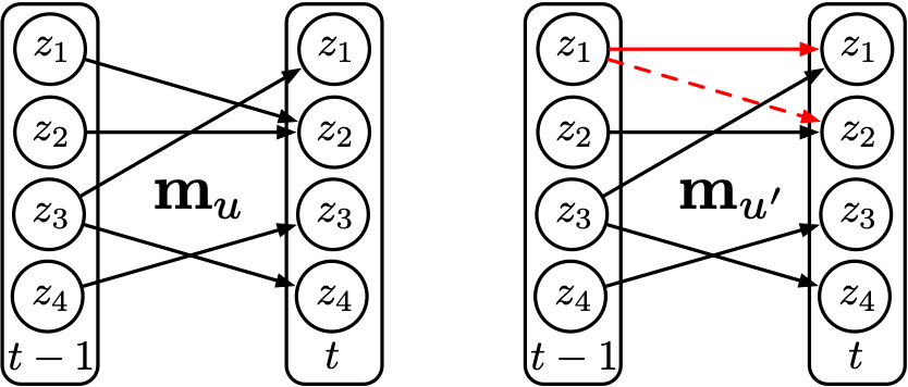
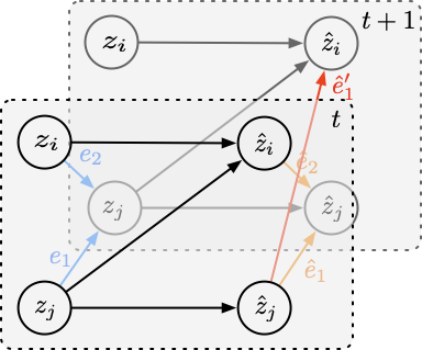
To make this precise, we need a measure of transition complexity. Recall that the transition \(\mathbf{z}_{t+1} = f(\mathbf{z}_t)\) acts component-wise: each latent dimension \(z_{t+1,i}\) may depend on only a subset of the dimensions in \(\mathbf{z}_t\). This forms a bipartite directed graph from \(\mathbf{z}_t\) to \(\mathbf{z}_{t+1}\), where each edge represents a direct dependency. We measure complexity by the number of edges in this graph — the fewer edges, the simpler (sparser) the transition. We further require that all transitions differ by at least one edge. For example, the figure below shows two different regimes \(u\) and \(u'\), with the differences highlighted in red.

Figure 2: Two different regimes $u$ and $u'$ with different transition structures.

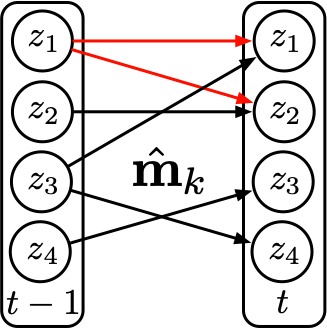
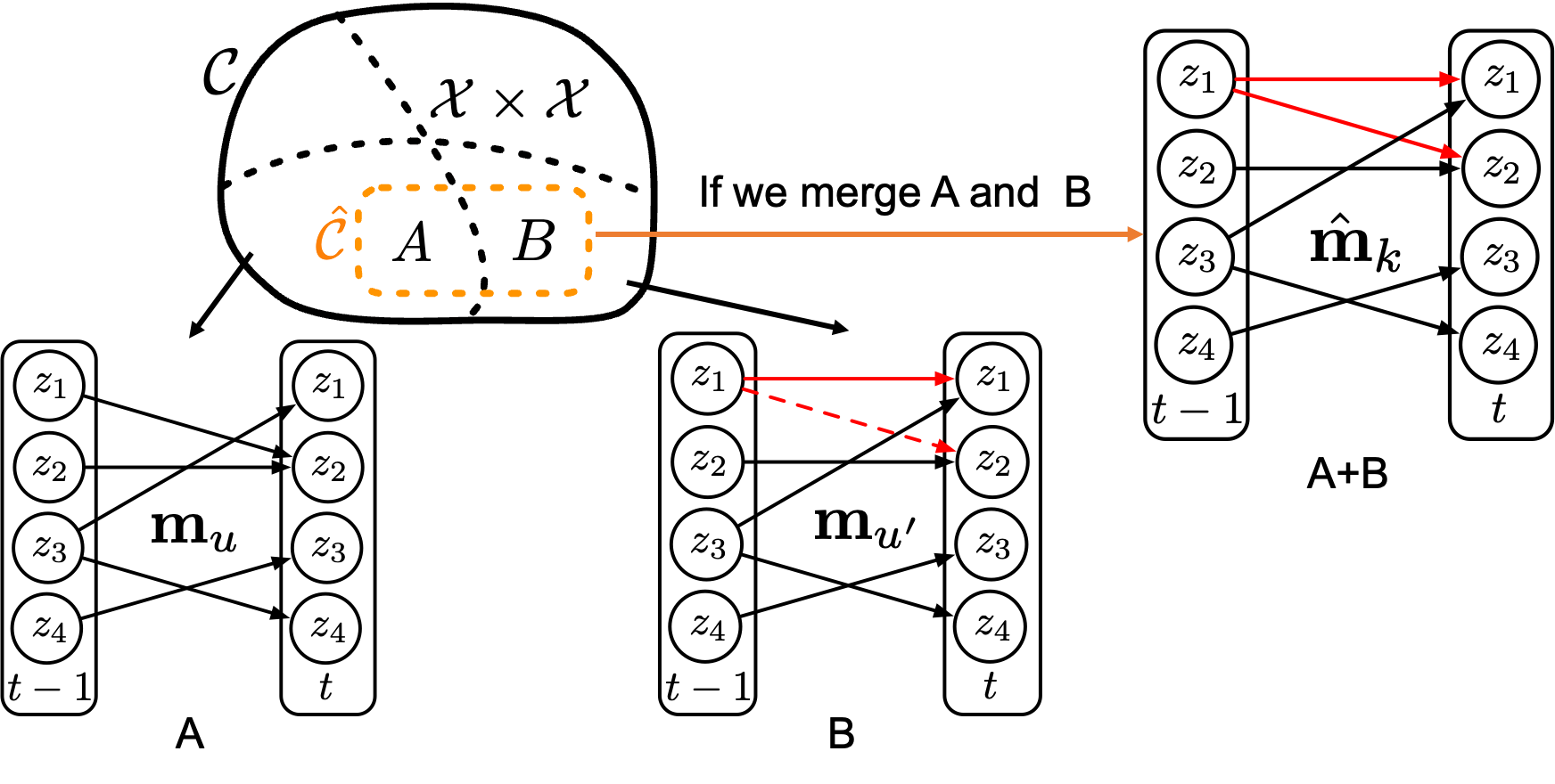
For two data points from these two regimes, if we assign correct regime labels, then we can learn two transition functions each with 5 edges, as shown in Figure 2. However, if we assign wrong regime labels — for example, assigning a unified regime \(k\) — then to fit the data, we need to learn a transition function that covers both the edges in regime \(u\) and the edges in regime \(u'\). This means the transition function will have at least 6 edges, as shown in Figure 3 below.

Figure 3: If we assign wrong regime labels, the learned transition function becomes more complex.

Therefore, from a distributional perspective, when we partition the dataset into different regimes and make mistakes, the support of the incorrectly partitioned region will always yield a more complex transition function than the correctly partitioned regimes. In other words, as long as we push the estimated transition functions to be as simple as possible, the predicted regime changes will be correct.

Figure 4: Dataset partitioning into different regimes. The correctly partitioned regimes yield simpler transition functions compared to incorrectly partitioned regimes.

What About Estimated Latent Variables?

A natural follow-up question: the complexity measure above is defined over the true latent space, yet in practice the latent variables are also estimated — how can we guarantee the complexity is measured correctly? The answer is that incorrectly estimating the latent variables (i.e., mixing up some of the dimensions) can only lead to more complex transition functions. As shown in Figure 5, if we mix up some dimensions in the latent space, we will need to add more edges to the transition function to fit the data, making the transition function more complex.

Figure 5: Incorrectly estimated latent variables lead to more complex transition functions.

Identifiability and Experimental Verification

By further applying the sufficient variability principle, we can guarantee the identifiability of the sequence model with nonstationary dynamics . The most interesting part is that, in theory, we first recover the regime changes and then apply the previous identifiability results to recover the latent variables and their causal graph within each regime. This two-stage process is clearly reflected in the estimation procedure.

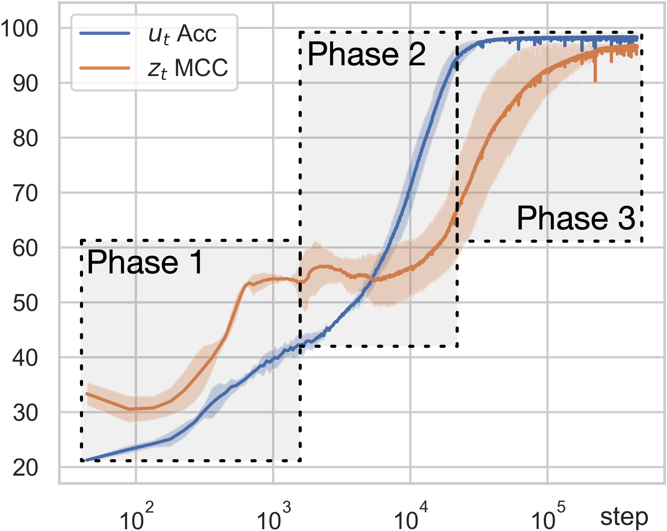
We use two evaluation metrics to measure estimation quality: the accuracy of the predicted regime changes (\(u_t\) Acc), and the Mean Correlation Coefficient (\(z_t\) MCC), which measures how well each estimated latent dimension aligns with a true latent dimension. As shown in Figure 6, the learning process unfolds in three distinct phases. In the first two phases, the accuracy of regime variables keeps increasing even though the MCC for latent variables remains very low — the model is learning to segment the sequence before it can recover the latent variables. Then in the third phase, the regime accuracy approaches 100% and the MCC for latent variables begins to increase significantly.

Figure 6: Estimation process for sequence models with nonstationary dynamics. The accuracy of predicted regime changes increases before the mean correlation coefficient of latent variables starts to improve, demonstrating a three-phase learning process.

Summary

We established an identifiability result for nonstationary sequential data with unknown distribution changes, using transition sparsity as the key inductive bias. The core argument is clean: wrong regime assignments or wrong latent representations both lead to denser transition graphs, so minimizing graph complexity jointly recovers the correct regimes and the correct latent variables. Synthetic experiments confirm this two-stage learning behavior, and the approach extends naturally to real-world tasks such as video segmentation. More broadly, this work shows how a principled formalization of Occam’s Razor — seeking the simplest explanation for observed dynamics — can turn human intuition into provable guarantees for causal representation learning.

Citation

If you found this post useful, please consider citing it:

@article{song2026seqmodel4,
  title={Sequence Model 4: Nonstationary Dynamics},
  author={Song, Xiangchen},
  year={2026},
  month={February},
  url={https://xiangchensong.github.io/blog/2026/seq-model-4/}
}