Sequence Model 2: Sufficient Variability

A family of assumptions that ensure identifiability in sequence models by leveraging sufficient variability in the latent dynamics.

Recap

In the previous post, we introduced sequence models from a causal representation learning perspective and highlighted the fundamental challenge of identifiability. We saw that a model can perfectly reconstruct observations while learning a completely meaningless internal representation—the classic “rotational ambiguity” of Variational Autoencoders (VAEs) being the simplest example.

However, we did not provide any concrete solutions. In this post, we will explore a powerful family of conditions called sufficient variability that can provably recover the true latent variables. The key insight is simple: if the statistical properties of latent variables change in “rich enough” ways across different contexts, we can tease apart the individual dimensions and identify them up to trivial ambiguities.

This post is based on a line of work starting from nonlinear ICA and culminating in recent advances in causal representation learning .

The Core Problem: When Are Two Representations “The Same”?

Before diving into solutions, let’s precisely formulate what we’re trying to achieve. Suppose the true data-generating process is:

\[\mathbf{z} \sim p(\mathbf{z}), \quad \mathbf{x} = g(\mathbf{z})\]

where \(\mathbf{z} \in \mathbb{R}^n\) are the true latent causal variables and \(g\) is an invertible mixing functionThe invertibility assumption ensures that no information is lost when mapping latents to observations. This is a strong but common assumption in the identifiability literature—without it, multiple latent configurations could produce identical observations, making recovery fundamentally impossible. that produces observations \(\mathbf{x}\). We want to learn an encoder \(\hat{g}^{-1}\) that recovers the latents from observations.

The trouble is that many different encoders can explain the same data equally well. Consider two data-generating processes:

Figure 1: Two data-generating processes that produce identical observations but use different latent representations.

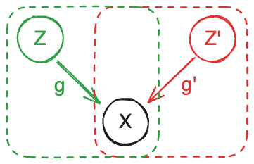
Both processes generate the exact same distribution over \(\mathbf{x}\). Since both decoders \(g\) and \(g'\) are invertible, we can express the relationship between the two latent representations as:

\[\mathbf{z} = h(\mathbf{z}') = g^{-1}(g'(\mathbf{z}'))\]

where \(h\) is the transformation mapping one representation to the other.

The identifiability question: Under what conditions must \(h\) be a “trivial” transformation?

Here, “trivial” typically means one of:

• Permutation: The recovered dimensions are the same as the true ones, just reordered
• Permutation + scaling: Each recovered dimension is a scaled version of a true dimension
• Permutation + element-wise transformation: Each recovered dimension \(\hat{z}_i = f_i(z_{\pi(i)})\) for some invertible \(f_i\) and permutation \(\pi\)

The last case—often called component-wise identifiabilityComponent-wise identifiability means we've recovered the "right" factors of variation. Monotonic transformations of each dimension are acceptable since they preserve ordering.—is usually what we aim for. It says we’ve correctly separated the latent dimensions; we just might have applied an invertible transformation to each one individually.

The Mathematical Tool: Jacobians

The Jacobian matrix captures how small changes in one set of variables affect another—think of it as a “sensitivity map” between representations.

To analyze when \(h\) must be trivial, we study its Jacobian matrix:

\[J = \frac{\partial \mathbf{z}}{\partial \mathbf{z}'} = \frac{\partial h(\mathbf{z}')}{\partial \mathbf{z}'}\]

The \((i,j)\) entry \(J_{ij} = \frac{\partial z_i}{\partial z'_j}\) measures how much the \(i\)-th true latent changes when the \(j\)-th recovered latent varies.

Key observation: If the Jacobian is a permutation matrixA permutation matrix has exactly one "1" in each row and column. When the Jacobian has this structure, each output is controlled by exactly one input—no mixing. (or can be permuted to be diagonal), then each true latent depends on exactly one recovered latent—and vice versa. This is precisely component-wise identifiability.

So our strategy becomes: find conditions under which the Jacobian of any valid transformation \(h\) must have this special structure.

Leveraging Independence

The fundamental constraint we exploit comes from independence. In many latent variable models, we assume the latent dimensions are (conditionally) independent:

\[p(\mathbf{z}') = \prod_{i=1}^{n} p(z'_i)\]

This factorial structure has a powerful consequence for the log-density:

\[\frac{\partial^2 \log p(\mathbf{z}')}{\partial z'_i \partial z'_j} = 0 \quad \text{for } i \neq j\]

The cross-derivatives of the log-density vanish for independent variables. This is because:

\[\log p(\mathbf{z}') = \sum_i \log p(z'_i)\]

and differentiating \(\log p(z'_i)\) with respect to \(z'_j\) gives zero when \(i \neq j\).

Now here’s the clever part. We can express this constraint in terms of the true latents \(\mathbf{z}\) using the change of variables$\log p(\mathbf{z}') = \log p(\mathbf{z}) + \log |J_h|$ from the change of variables formula. Differentiating both sides twice and using the product rule yields the three-term expression. and applying the chain rule, we get:

\[\frac{\partial^2 \log p(\mathbf{z}')}{\partial z'_i \partial z'_j} = \sum_{k} \frac{\partial \log p(\mathbf{z})}{\partial z_k} \frac{\partial^2 z_k}{\partial z'_i \partial z'_j} + \sum_{k} \frac{\partial^2 \log p(\mathbf{z})}{\partial z_k^2} \frac{\partial z_k}{\partial z'_i} \frac{\partial z_k}{\partial z'_j} + \frac{\partial^2 \log |J_{h}|}{\partial z'_i \partial z'_j} = 0\]

This equation must hold for all \(i \neq j\) and for all values of \(\mathbf{z}'\).

Note that if we make \(\frac{\partial z_k}{\partial z'_i} \frac{\partial z_k}{\partial z'_j}\) in the second term always zero for all \(i \neq j\), then for a given dimension \(k\), at most one of the partial derivatives \(\frac{\partial z_k}{\partial z'_i}\) can be non-zero. Equivalently, each row of the Jacobian has at most one non-zero entry, meaning each true latent \(z_k\) depends on at most one recovered latent \(z'_i\)—exactly what we need for component-wise identifiability.

Each Jacobian row represents one true latent. A single non-zero entry per row means a clean one-to-one correspondence with recovered latents.

Now consider the first term. This term poses no issue: if \(z_k\) depends on only one \(z'_i\), then its second derivative with respect to any other \(z'_j\) vanishes. The difficulty arises from the third term, which involves the log-determinant of the Jacobian. This term couples all partial derivatives together, making direct analysis challenging.

Introducing Auxiliary Variables

One way to eliminate the troublesome third term is to find two such equations that share the same Jacobian and subtract them, so that the log-determinant terms cancel out. Since the Jacobian \(h\) depends only on \(\mathbf{z}'\) (not on \(\theta\)), the log-determinant term is identical for both equations and cancels when we subtract. This is what we call auxiliary variables or domain variables.

Assuming the independence constraints hold given a domain variable \(\theta\), we take the difference between two different values: \(\theta^{(u)}\) and \(\theta^{(0)}\) (where \(u\) indexes different domain values, e.g., \(u = 1, 2, \ldots\)). This eliminates the troublesome term and yields a cleaner equation:

\[\sum_{k} \left(\Delta \frac{\partial \log p(\mathbf{z}; \theta^{(u)})}{\partial z_k} \frac{\partial^2 z_k}{\partial z'_i \partial z'_j}\right) + \sum_{k} \left(\Delta \frac{\partial^2 \log p(\mathbf{z}; \theta^{(u)})}{\partial z_k^2} \frac{\partial z_k}{\partial z'_i} \frac{\partial z_k}{\partial z'_j}\right) = 0\]

where \(\Delta \frac{\partial \log p(\mathbf{z}; \theta^{(u)})}{\partial z_k} = \frac{\partial \log p(\mathbf{z}; \theta^{(u)})}{\partial z_k} - \frac{\partial \log p(\mathbf{z}; \theta^{(0)})}{\partial z_k}\), and similarly for the second derivative. Now there are a total of \(2n\) unknowns:

\[\Delta \frac{\partial \log p(\mathbf{z}; \theta^{(u)})}{\partial z_k}, \quad \Delta \frac{\partial^2 \log p(\mathbf{z}; \theta^{(u)})}{\partial z_k^2}, \quad k = 1, \ldots, n\]

That leads us to the sufficient variability assumption, which roughly states that we need at least \(2n + 1\) different values of \(\theta\) such that the changes in those derivatives are linearly independent. Intuitively, this means the latent distribution must change in sufficiently diverse ways across domains—no single domain’s change can be expressed as a linear combination of changes from other domains. With enough such independent variations, the system of equations becomes sufficiently constrained that the only solution is to have each \(\frac{\partial z_k}{\partial z'_i} \frac{\partial z_k}{\partial z'_j} = 0\) for all \(i \neq j\), which gives us component-wise identifiability.

The choice of auxiliary variables is flexible—they can be discrete domain indices, continuous conditioning variables, or even time indices in sequential data. In the next posts, we will see how to choose them in sequence models to satisfy the sufficient variability assumption and achieve provable identifiability of the latent dynamics.

Citation

If you found this post useful, please consider citing it:

@article{song2026seqmodel2,
  title={Sequence Model 2: Sufficient Variability},
  author={Song, Xiangchen},
  year={2026},
  month={February},
  url={https://xiangchensong.github.io/blog/2026/seq-model-2/}
}