Sequence Model 1: Identifiability

An introduction to sequence models through the lens of causal representation learning and the fundamental challenge of recovering latent truth.

Motivation

Sequence models are the backbone of modern AI, from the humble RNN to the ubiquitous Transformer. But when we talk about a “sequence,” what are we actually modeling?

In most deep learning contexts, we treat sequences as a stream of observations where we minimize prediction error:

\[\min_{\theta} \sum_{t=1}^{T} \|\mathbf{x}_t - h_\theta(\mathbf{x}_{\lt t})\|^2\]

where \(h_\theta\) is our predictor that takes past observations \(\mathbf{x}_{\lt t}\) and predicts the next observation \(\mathbf{x}_t\). (For simplicity, we write a squared-error objective, though the same argument applies to probabilistic losses like cross-entropy or negative log-likelihood.)

The problem with this approach is that if we only model the raw observations, the mapping \(h_\theta\) from the past to the future becomes incredibly complex.

Example: Consider a video of a moving pendulum. If we try to predict the next frame \(\mathbf{x}_{t+1}\) directly from the current frame \(\mathbf{x}_t\), we are trying to learn a function over thousands of high-dimensional pixels. This function must account for lighting, texture, and background—most of which are irrelevant to the pendulum’s motion.

Figure 1: Comparison between predicting in high-dimensional observation space (pixels) versus low-dimensional latent space (causal variables). Recovering the underlying state simplifies complex dynamics into predictable physical laws.

Figure credits to Nano Banana Pro.

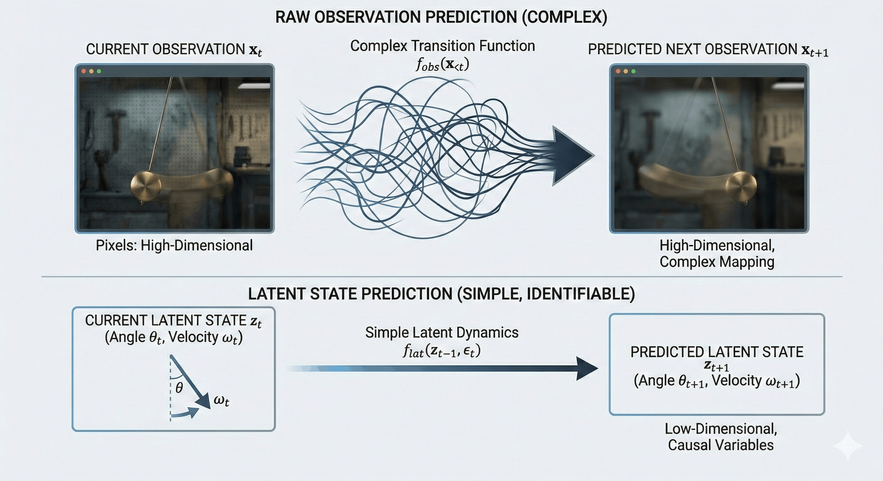
However, if we model the underlying variables that actually control the data generation process—the angle and angular velocity—the “future” becomes much simpler to predict.

This suggests that prediction is not the right primitive. Instead, we should model the data-generating process itself. This is why, in causal representation learning, we view sequence models as dynamic systems driven by hidden causal variables. This perspective connects sequence models to classic system identification and recent work on nonlinear ICA with auxiliary variables.

The Causal View

Figure 2: Graphical model of the data-generating process.

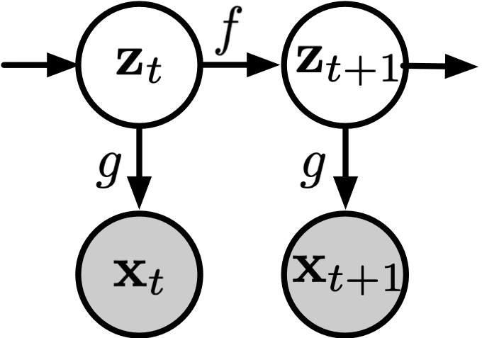
From a causal perspective, a sequence model consists of two fundamental components:

1. Latent Dynamics (\(f\)): At each time step \(t\), the hidden state \(\mathbf{z}_t\) evolves from its previous value: \(\mathbf{z}_t = f(\mathbf{z}_{t-1}, \epsilon_t)\) Here, \(\mathbf{z}_t = \{z_{t,1}, z_{t,2}, \dots, z_{t,n}\}\) represents the true causal variables (e.g., position and velocity), and \(\epsilon_t\) is independent noise driving the system. (The properties of \(\epsilon_t\)—such as independence and distributional assumptions—will turn out to be crucial for identifiability, a point we return to in the next post.)

2. Observation Function (\(g\)): We never observe \(\mathbf{z}_t\) directly. Instead, we see a high-dimensional observation: \(\mathbf{x}_t = g(\mathbf{z}_t)\) This mapping \(g\) “entangles” the clean latent variables into messy, high-dimensional data like pixels or text tokens.

The key insight is that if we can recover the true latent variables \(\mathbf{z}_t\) from observations \(\mathbf{x}_t\), prediction becomes trivial—we just need to model the simple dynamics \(f\) rather than the complex observation-to-observation mapping \(h_\theta\). To make this contrast explicit:

\[\text{Observation space:} \quad \mathbf{x}_t = h(\mathbf{x}_{\lt t})\] \[\text{Latent space:} \quad \mathbf{z}_t = f(\mathbf{z}_{t-1}), \quad \mathbf{x}_t = g(\mathbf{z}_t)\]

But here lies the fundamental challenge: can we actually recover these latent variables? Here, “recover” means identifying the latent variables up to unavoidable equivalences (e.g., permutation or component-wise transformation), not exact numerical equality.

The short answer is: not always.

The Identifiability Crisis

Just because a model reconstructs \(\mathbf{x}_t\) perfectly does not mean it has discovered the true \(\mathbf{z}_t\). This is the problem of identifiability—without the right constraints, infinitely many “wrong” representations can explain the same data equally well.

In practice, this means a sequence model can achieve near-perfect prediction while internally representing the world in a way that is physically meaningless.

Consider a standard Variational Autoencoder (VAE) with an isotropic Gaussian prior on \(\mathbf{z}\). Here, the model learns to map the data distribution \(p(\mathbf{x})\) into the latent space. However, because Gaussians are rotationally symmetric, any rotation \(\mathbf{R}\) of the latent space leaves the prior density \(p(\mathbf{z})\) completely unchanged. This creates a mathematical “blind spot”: the model has no incentive to prefer the true causal orientation over any arbitrary rotation. It might reconstruct the observations perfectly, yet fail to disentangle meaningful features—leaving “position” and “velocity” inextricably mixed.

This is the classic rotational ambiguity problem. In the i.i.d. setting, VAEs are fundamentally unidentifiable because the Gaussian prior cannot "pin down" the coordinate axes. The example was first discussed in .

This raises two critical questions for sequence models:

1. Can we leverage temporal structure—the fact that \(\mathbf{z}_t\) depends on \(\mathbf{z}_{t-1}\)—to break this symmetry?
2. Under what conditions can we guarantee that the learned representation matches the true causal variables?

Unlike the i.i.d. setting, temporal data contains asymmetries—time, causation, and noise propagation—that may partially break these symmetries.

In the next post, we will show that under some mild conditions, temporal structure can act as supervision—turning prediction into identification.

Citation

If you found this post useful, please consider citing it:

@article{song2026seqmodel1,
  title={Sequence Model 1: Identifiability},
  author={Song, Xiangchen},
  year={2026},
  month={January},
  url={https://xiangchensong.github.io/blog/2026/seq-model-1/}
}